Green Energy + AI: Building Predictive Smart HEMS with EMQ Device Agent


Driven by global decarbonization goals and power market deregulation, residential energy storage is evolving from a passive power bank into a self-optimizing financial asset. The core driver behind this evolution is AI.
This article explores how to build an intelligent Home Energy Management System (HEMS) using the EMQ Device Agent and IoT Platform. The system understands natural language commands, forecasts future power generation and consumption, and calculates optimal charging and discharging schedules. Detailed engineering insights and real-world benchmark data for the underlying forecasting algorithms are also provided.
Background: The Imperative of the Dynamic Tariff Era
For home energy storage products operating in competitive international markets, "Green Energy + AI" is no longer an optional add-on; it is a ticket to entry. Wholesale electricity spot markets increasingly settle on 15-minute intervals. With the rapid adoption of dynamic tariff contracts (such as those from Tibber and Octopus Energy across Europe), residential electricity prices fluctuate hourly or even every 15 minutes based on grid supply and demand.
This fundamentally shifts the value proposition of residential energy storage: moving from passive solar self-consumption to active energy arbitrage — charging when grid power is cheap (or negatively priced) and discharging during peak price hours. Faced with high-frequency price fluctuations, static, schedule-based charging profiles fail completely. Predictive forecasting and dynamic optimization have become absolute necessities.
Ultimately, customer requirements converge on a single core technical challenge:
How to predict future energy consumption and solar generation based on historical load, historical PV generation, weather data (irradiance, temperature, humidity, wind speed), and 15-minute electricity tariffs, and dynamically determine the optimal battery dispatch plan accordingly.
Furthermore, solutions must deliver per-household personalization. Because power consumption habits vary drastically from home to home, generic profile templates cannot handle real-world operational demands.
Challenges: AI as the Core and the Hurdle
The technical complexity of this scenario is heavily concentrated in the AI layer across two primary dimensions:
- Optimization Algorithms: Every household possesses a unique load profile that requires targeted learning and validation using complete historical telemetry. Furthermore, models must continuously iterate as new data accumulates rather than remaining static after deployment.
- User Experience: Advanced algorithmic capabilities must be delivered frictionlessly to end-users. Users should be able to customize workflows through natural language (such as setting ad-hoc timers, adjusting parameters, or querying historical telemetry) without navigating complex configuration forms.
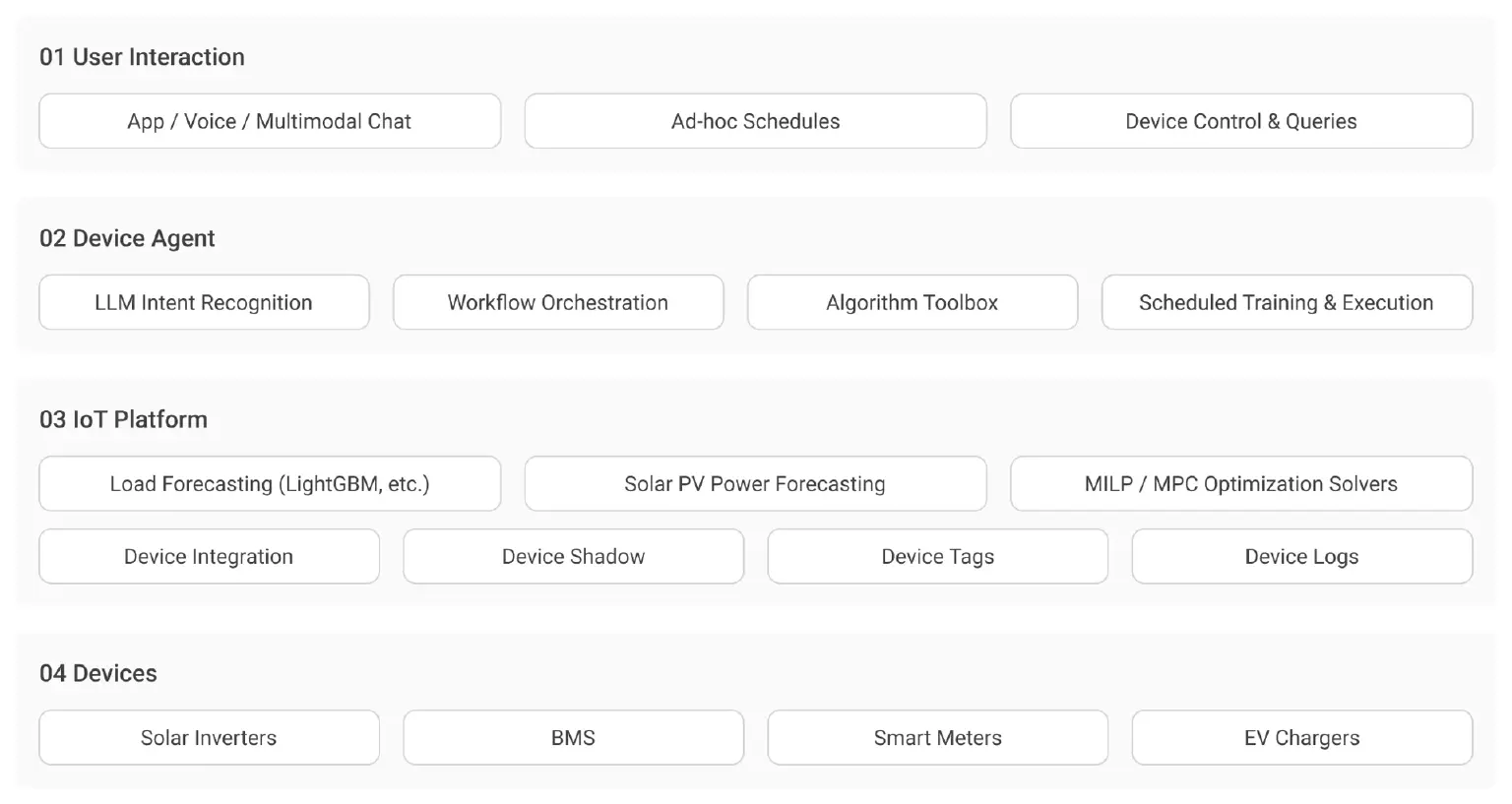
Foundation: Device Agent + IoT Platform
The solution is built on a two-layer foundation:
- The upper layer (Device Agent) enables rapid agent capability deployment.
- The lower layer (IoT Platform) manages device connectivity and data asset management.
Device Agent: Rapid DER Agent Development
- Device Onboarding & Conversational Interface: Provides device integration, Device Models, and multimodal conversation capabilities, enabling solar inverters, energy storage batteries, and smart meters to become interactable via natural language.
- Workflow & Algorithm Integration: Mounts predictive models and optimization solvers as "Tools" attached to the agent. This decouples algorithm iteration from the conversational interaction layer, allowing flexible orchestration on demand.
IoT Platform: Connectivity & Asset Management
- Lifecycle Management: Delivers device provisioning, tagging, logging, and device shadow capabilities to ensure operational reliability across the hardware lifecycle.
- Data Asset Storage & Retrieval: Stores and queries historical data, including consumption, generation, and weather telemetry. Structured data serves as the fuel for AI models, where data integrity directly dictates the precision upper bound of personalized algorithms.
Architecture: LLM × Predictive Model × Solver
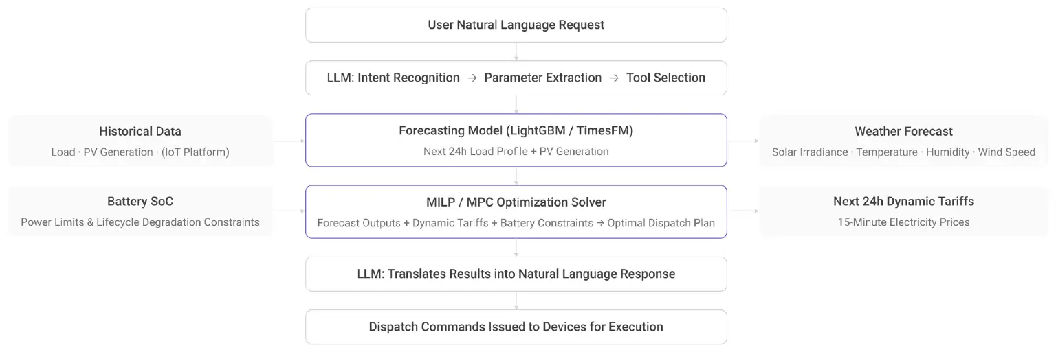
The system operates through a decoupled three-stage pipeline:
- LLM: Interprets natural language, performs reasoning, and generates conversational feedback.
- Forecasting Model: Predicts future load profiles and solar generation based on historical telemetry and real-time weather data.
- Optimization Solver: Calculates the optimal charge/discharge schedule under strict physical constraints.
Any single module can be independently upgraded without disrupting the broader pipeline.
Load & Solar Forecasting Algorithms
Balanced Mode via LightGBM
Forecasting approaches range from classic machine learning algorithms to Time-Series Foundation Models (TSFMs). In our architecture, LightGBM is selected to implement the "Balanced Mode." Using the public UCI Appliances Energy Prediction dataset (19,735 records sampled at 10-minute intervals), we highlight key engineering considerations:
Feature Engineering is Paramount:
- Cyclical Time Features: Hour and day-of-week encoded using Sine/Cosine transformations (ensuring the model recognizes that hour 23 is adjacent to hour 0), augmented with coarse time-of-day binning.
- Multi-Scale Lag Features: Historical power consumption and outdoor climate metrics lagged from 10 minutes to 24 hours to capture load inertia.
- Rolling Window Statistics: Moving averages and standard deviations over 1-hour, 4-hour, and 24-hour windows to capture short-term usage levels and volatility.
Strict Chronological Data Splitting:
Data is split strictly in temporal sequence (70% training, 30% testing). Random shuffling is avoided entirely to prevent future data leakage, one of the most common pitfalls in time-series modeling.
Benchmark Performance:
Running the pipeline on the benchmark dataset (learning_rate=0.03, num_leaves=63, early stopping) yields the following results:
| Metric | LightGBM | Naive Baseline (Same Time Yesterday) |
|---|---|---|
| RMSE | 60.34 Wh | 111.64 Wh |
| Relative Improvement | ~46% reduction | — |
The top 10 most impactful features are dominated by lag variables and rolling window statistics (followed by indoor humidity and hourly cyclical encodings). This confirms that historical consumption patterns provide the strongest signal for load forecasting, with weather metrics serving as vital supplementary inputs.
From Sample Code to Production: Bridging Four Gaps
Validation on a public dataset is only a starting point. Deploying to production requires addressing four critical engineering gaps:
- Integrating Solar Generation Forecasting: Public datasets often contain only household electrical load. Production environments require a dual-model setup (Load + Solar Generation), where solar irradiance serves as the primary driver for PV modeling.
- Moving from Single-Step to Multi-Horizon Forecasting: Sample scripts often use actual lagged values to predict the single next step. Production requires predicting 96 steps ahead (a full 24-hour horizon at 15-minute intervals) using direct multi-horizon forecasting (substituting forecasted weather features for actuals) or recursive forecasting.
- Time-Resolution Alignment: Raw telemetry may arrive at 10-minute intervals, whereas electricity tariffs and battery dispatch schedules operate on 15-minute blocks. Data must be resampled and aligned accordingly.
- Incorporating Tariff Features: Because arbitrage is central to HEMS, historical and forward-looking tariff rates must be integrated directly into training features.
Engineering Note: In basic scripts, early stopping validation is often run directly on the test set. In production, a distinct validation split must be carved from the tail end of the training set. Correcting for this yields a realistic RMSE estimate of 63.15 Wh. Note also that
root_mean_squared_errorrequiresscikit-learn >= 1.4.
Alternative Algorithm Options
- XGBoost: Belongs to the same gradient boosting tree family as LightGBM; serves as a natural benchmark or ensemble candidate.
- Linear Regularization (ElasticNet / Ridge): Achieves precision within 1% of LightGBM (RMSE difference < 1%). Ideal as a lightweight, production-grade baseline deployed directly on local storage gateways, or as a reference baseline for anomaly detection.
- Neural Networks: Provide advantages when performing joint multi-household training over massive datasets.
- Time-Series Foundation Models (e.g., Google TimesFM 2.5): Pre-trained on vast time-series corpora, TSFMs solve the "cold-start" problem. For new users lacking historical data, TimesFM delivers a robust baseline forecast. Once sufficient data accumulates (e.g., 4+ weeks), the system seamlessly transitions to a personalized LightGBM model, creating a feedback loop with out-of-the-box accuracy that improves over time. (Note: TSFMs require GPU infrastructure, introducing higher compute overhead.)
Three Energy Management Modes: One Framework, Distinct Objectives
The solution offers three standard operating modes: Balanced, EMS, and Eco-Friendly. These are not separate standalone algorithms, but rather different weight configurations applied to the same objective function within a unified optimization solver:
| Mode | Objective Function Focus | Target User Profile |
|---|---|---|
| Balanced Mode | Arbitrage Revenue − Battery Degradation Cost (factors battery cycle wear into the objective) | Standard households balancing financial returns with battery longevity |
| EMS Mode | Maximizes pure arbitrage profit; permits deeper Depth of Discharge (DoD) and aggressive dispatch schedules | Users seeking maximum financial returns with sufficient battery warranty margin |
| Eco-Friendly Mode | Maximizes PV self-consumption rate; reduces weight on economic arbitrage | Users prioritizing carbon footprint reduction and energy self-reliance |
Under this design, adding a new operational mode simplifies to introducing a new weight configuration set rather than engineering a new algorithm from scratch.
Model Training & Tooling
Training Pipeline: Personalized & Scheduled
- Inputs: Historical load telemetry, solar generation data, and weather logs fetched from the IoT Platform (isolated per User ID).
- Outputs: A personalized 24-hour forecasting model tailored to the household and selected mode.
- Frequency: Each user is modeled independently. The Device Agent automatically triggers weekly retraining to continuously capture seasonal shifts and changing usage habits.
Device Agent Tooling Interface
Algorithms are exposed on the IoT Platform as standard tools accessible via REST/gRPC APIs, enabling the Device Agent to invoke them within conversational workflows:
| Tool | Parameters | Function / Output |
|---|---|---|
| Create / Update Training Pipeline | User ID, Mode Type | Trains and updates the personalized forecasting model for the target user. |
| Invoke Optimization Solver (MILP / MPC) | User ID, Mode Type, Current Battery SoC, 24h Weather Forecast, 24h Tariff Schedule | Computes and returns the optimal 24-hour charge/discharge plan. |
Safety & Reliability Guardrails
Because charge and discharge commands actuate physical hardware, safety guarantees are critical. The system enforces guardrails across three distinct tiers:
- Hard Constraints: SoC upper/lower bounds, maximum charge/discharge rates, and thermal limits are enforced as unalterable hard constraints in the optimization solver (e.g., MILP/MPC), not soft penalties. AI optimizes within these bounds and can never cross them.
- Human-in-the-Loop Confirmation: High-impact operations (e.g., mode toggling, manual overrides) require explicit user approval before execution.
- Deterministic Fail-Safe Fallbacks: If forecasting services, solvers, or cloud connectivity experience anomalies, the gateway automatically falls back to a deterministic local execution rule (e.g., default solar self-consumption).
Core Principle: The LLM does not control hardware directly. All dispatches must pass through deterministic optimization solvers and hardware safety validation.
Real-World Interaction Workflows
Scenario 1: User says, "Set my battery to EMS Mode."
- Agent inspects Skills -> Identifies "Create / Update Training Pipeline" tool.
- Agent schedules weekly retraining for user's EMS model.
- Agent establishes hourly cron job to run Solver & update dispatch plans.
- Agent replies to User: "Switched to EMS Mode. Your schedule will optimize hourly based on real-time tariffs and weather forecasts."
Scenario 2: User says, "I have guests coming over this afternoon, please adjust today's plan."
- Agent infers higher afternoon load demand.
- Agent adjusts inputs: Boosts load forecast offset & raises minimum evening SoC reserve limit.
- Agent triggers immediate re-solve -> Generates revised 24h plan.
- Agent replies: "Adjusted for guests today: Afternoon power will be prioritized, battery will pre-charge during solar peak, holding 40% SoC for evening use."
This capability demonstrates the core distinction between a Device Agent and a traditional EMS: the LLM translates ad-hoc natural language intent into real-time adjustments of mathematical solver parameters and operational constraints, rather than relying on rigid static presets.
Financial ROI & Performance Evaluation
Forecasting accuracy translates directly into financial utility. The economic evaluation framework is defined as:
Electricity Cost Savings = Σ (Discharged Energy × Tariff Rate at Discharge) − Σ (Charged Energy × Tariff Rate at Charge) − Battery Degradation Cost
Two process indicators accompany this monetary evaluation: PV Self-Consumption Rate and Peak Tariff Coverage Ratio. Mode performance comparisons should be validated via backtesting: applying actual historical consumption, PV generation, and tariff time-series data to simulate dispatches across all three modes.
The relationship between forecasting accuracy and financial return is monotonic: lower forecasting error directly reduces costly misalignments (e.g., failing to charge during low price windows or discharging prematurely). The LightGBM benchmark's 46% RMSE reduction over the naive baseline translates directly to eliminating the majority of dispatch misalignments, delivering the core economic value of AI over static rules.
Summary
AI does not replace traditional EMS; it augments them with three critical capabilities:
- Conversational Interface: LLMs translate mathematical optimization capabilities into plain-language interactions.
- Market Adaptability: Predictive models convert historical telemetry into forward-looking decisions that react to dynamic tariffs.
- Scalable Personalization: Optimization solvers (MILP/MPC) make ideal dispatch decisions within strict physical safety constraints for every individual household.
The layered architecture combining a Device Agent with an IoT Platform moves smart home energy management from custom project implementations to scalable, productized deployments. Algorithms plug in as modular tools, operational modes scale via parameter weightings, and models evolve automatically on a scheduled basis.
Ready to transform your energy assets with Next-Gen AI?
Explore our Device Agent: Device Agent - Turn Any IoT Device into an AI Agent