What a PV Cooling Paper Reveals About Distributed IoT Control

Introduction

A 600 Wp experimental PV installation in the Czech Republic ran for 52 days in the field with active water cooling. Over that period, the cooling produced more extra electricity than the pumping system consumed: an Energy ROI of 1.07 on representative high-irradiance days. That's unusual. Most active PV-cooling studies describe pumps that eat more electricity than the cooling saves, even when the peak-gain numbers look attractive.

Novak and Landkamer's new paper in Energy Conversion and Management: X explains where the positive balance comes from. The cooling hardware isn't new: Kuo and Lo published on active water cooling back in 2013, and pv magazine recently framed this paper as moving the technology "closer to commercial viability." What's new is a control algorithm that learned to skip cooling when rain was about to do the job for free.

This post is about why that algorithm is inseparable from the distributed architecture that runs it. The control algorithm and the edge/fog layout that carries it are two views of the same structural property. The architecture is the algorithm.

The Experiment Setup

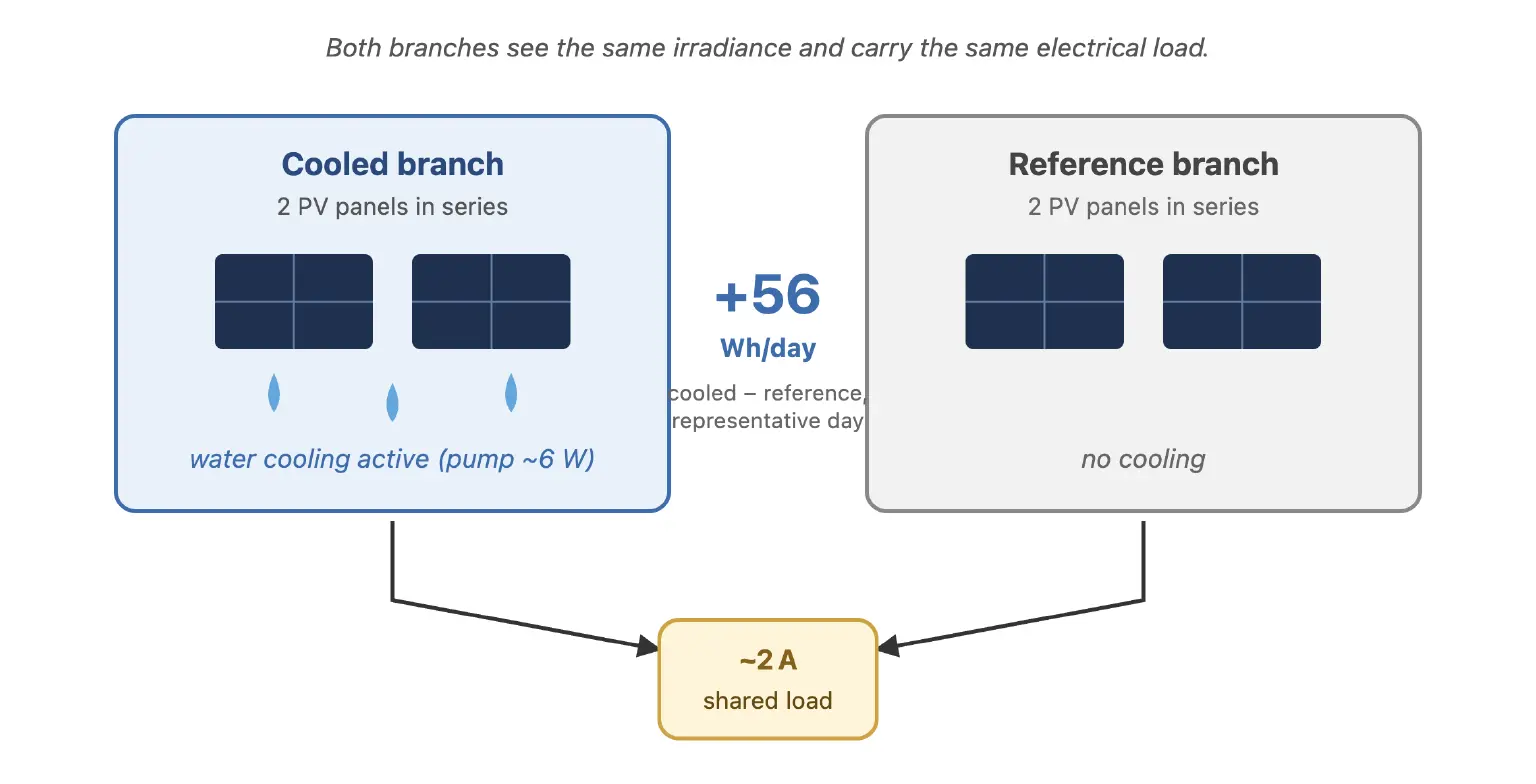
Novak and Landkamer tested cooling with a matched-pair design: two parallel branches of PV panels running side by side, one water-cooled and one as an uncooled reference. Both branches see the same sunlight and power the same constant electrical load, so any difference in their daily energy output is attributable to the cooling effect alone.

The field test ran for 52 valid daylight days across spring through early fall 2024. Each branch held two PV panels in series, with a 600 Wp rating per branch.

What the Paper Measured

On a representative high-irradiance day, the cooled branch produced about 56 Wh more electricity than the reference. The pump drew 6.0 W while active, consuming about 53 Wh over the day. Divide the extra energy by the pump's consumption and the Energy ROI is 1.07: the cooling generated slightly more electricity than the pumping consumed.

Across all 52 days, the mean daily gain was 5.84% (95% CI 5.04%, 6.65%), with peak daily gains of 7.38% on high-irradiance days. Total instantaneous control-side load (ESP32 edge nodes + Raspberry Pi fog + pump) never exceeded 10 W, under 2% of the branch's 600 Wp nominal rating.

These numbers are solid but not remarkable on their own; many cooling studies report similar peak gains. In §4.4, the authors compare the implemented weather-aware adaptive strategy against a reconstructed temperature-threshold baseline using the same 52-day dataset.

The Weather-Aware Strategy is Doing the Work

The comparison:

• Temperature-threshold baseline (the first-draft design): run the pump whenever panel temperature exceeds a cutoff.
• Weather-aware adaptive strategy (what they actually shipped): run the pump only when temperature exceeds the cutoff and a short-term weather outlook (fused from barometric pressure trends and AS3935 lightning activity) doesn't indicate imminent precipitation.

With the adaptive strategy, the pump ran 18–27% less than it would have under the threshold-only baseline. On storm-transition days, 30% less. And despite the pump running much less, the daily energy gain dropped by under 10%. The strategy was selectively skipping pump activations that wouldn't have paid off, because the panel would cool passively within hours anyway, once the rain arrived.

The paper doesn't compute this next step explicitly, but the arithmetic follows from the daily numbers above. A threshold-only baseline would consume roughly 20% more pump energy (~63 Wh/day instead of 53) for about 10% more gain (~62 Wh/day instead of 56). Plug those into the ROI formula and the baseline lands somewhere between 0.92 and 1.00.

Without the weather-aware suppression, this would have been yet another cooling system that consumes more than it recovers. pv magazine's "closer to commercial viability" framing is, at the technical core, an algorithmic story rather than a hardware one.

How the Algorithm Works

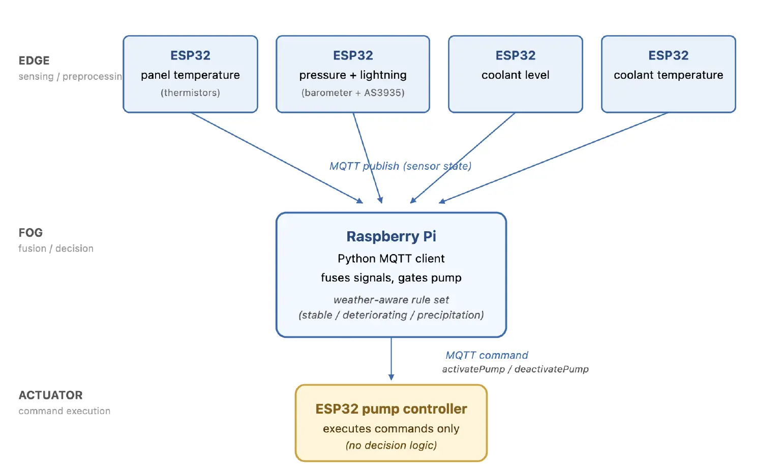
The algorithm has three pieces, each running on a different class of hardware.

Edge: Weather Sensing on Its Own ESP32

A dedicated ESP32 runs a barometric pressure sensor and ams OSRAM's AS3935 Franklin lightning detection IC.

• Pressure: sampled every 5 seconds, averaged over 30-minute windows. The node keeps a rolling 3-hour buffer of seven averaged samples and computes the gradient as a discrete temporal derivative.
• Lightning: treated as a multi-state indicator (near / distant / idle), not a binary event.

The two signals fuse locally into a compact categorical output: stable, deteriorating, or probable precipitation. That category is the only thing this edge publishes over MQTT. The raw pressure samples never leave the node.

Fog: Decision-Making on a Raspberry Pi

A Raspberry Pi running a Python MQTT client subscribes to four inputs:

• The weather state, from the weather edge node.
• Panel surface temperature, from a separate ESP32 with thermistors calibrated via the Steinhart-Hart equation.
• Coolant reservoir level.
• Coolant temperature.

A rule set gates pump activation: every condition must indicate cooling is needed now and not about to be made redundant by incoming precipitation. If yes, the fog publishes activatePump. Otherwise, deactivatePump.

Actuator: Command Execution Only

The pump's ESP32 subscribes to activation commands and executes them. No decision logic lives at this layer.

Three Properties That Shape What the Architecture Must Do

The algorithm is structured:

1. Multi-signal. Panel temperature, ambient air, humidity, barometric pressure, lightning events, coolant level, coolant temperature. Each sensor has its own placement, sampling rate, and failure mode.
2. Multi-location. Panel thermistors on the panels. Ambient sensors in ambient air. The lightning detector placed to see RF sferics without switching noise. Coolant sensors in the reservoir. No single mounting location holds them all.
3. Multi-timescale. 5-second edge sampling. 30-minute pressure averaging. 3-hour gradient windows. Per-event lightning processing. Pump decisions within a minute of threshold crossing. That's several orders of magnitude in one algorithm.

These three properties are what the architecture has to carry.

Why the Architecture Fits the Algorithm

A single-microcontroller implementation is possible in principle: long wires from every sensor to a central MCU, ADC multiplexing, per-signal timers, one fused control loop, and a pump relay at the end. The same authors built exactly that in their 2023 paper in Renewable and Sustainable Energy Reviews. The new paper is explicitly an argument against that design.

What goes wrong in the single-MCU version:

• Wiring and noise. Long analog cable runs pick up EMI, degrade accuracy, and constrain where sensors can sit. The paper observes that centralized control "increases wiring complexity, and restricts the number of deployable sensors."
• Extensibility. Adding a signal means a new cable, a re-flash, and a regression test of the whole system. With the MQTT layout: "New nodes simply register as MQTT clients within the predefined topic structure."
• Failure isolation. A corroded connector or shorted cable in any signal path can cascade into the central controller and corrupt the fused state. No compartmentalization.
• Timescale coupling. One clock, forcing the system either to over-sample signals that don't need it or to miss signals that do.

The three-layer split addresses each of these:

• Edge. One sensor (or a tight group), one node, one power budget per ESP32. Local calibration and preprocessing happen on the node. A failed edge node drops its own signal and nothing else. Adding a new signal = new ESP32 + new topic.
• Fog. The Raspberry Pi subscribes to signals it needs and fuses them at the cadence it needs them, independent of how fast any edge is sampling. Python on a general-purpose OS is good ground for evolving logic.
• Actuator. The pump's ESP32 executes received commands. Control logic lives elsewhere, so changes don't touch field hardware.
• MQTT as the only coupling. No bus wiring, no shared clock, no shared memory. Topics are the interface between layers.

The three properties of the algorithm map directly onto architectural primitives:

• Multi-signal → pub/sub fan-in.
• Multi-location → physical distribution of independent nodes.
• Multi-timescale → independent liveness with per-node timers.

The algorithm and the architecture are the same structural properties in two different vocabularies: one about information flow, one about hardware layout.

The Argument is About the Pattern, Not the Protocol

None of this is MQTT-specific. The paper describes its communication layer as "Wi-Fi or, alternatively, LoRaWAN for long-range low-power operation," and the same topology works over CoAP with its Observe extension or AMQP 1.0. What's load-bearing is the lightweight pub/sub with a broker pattern. MQTT happens to be the canonical IoT instance, which is why the paper uses it. The structural argument is about the pattern.

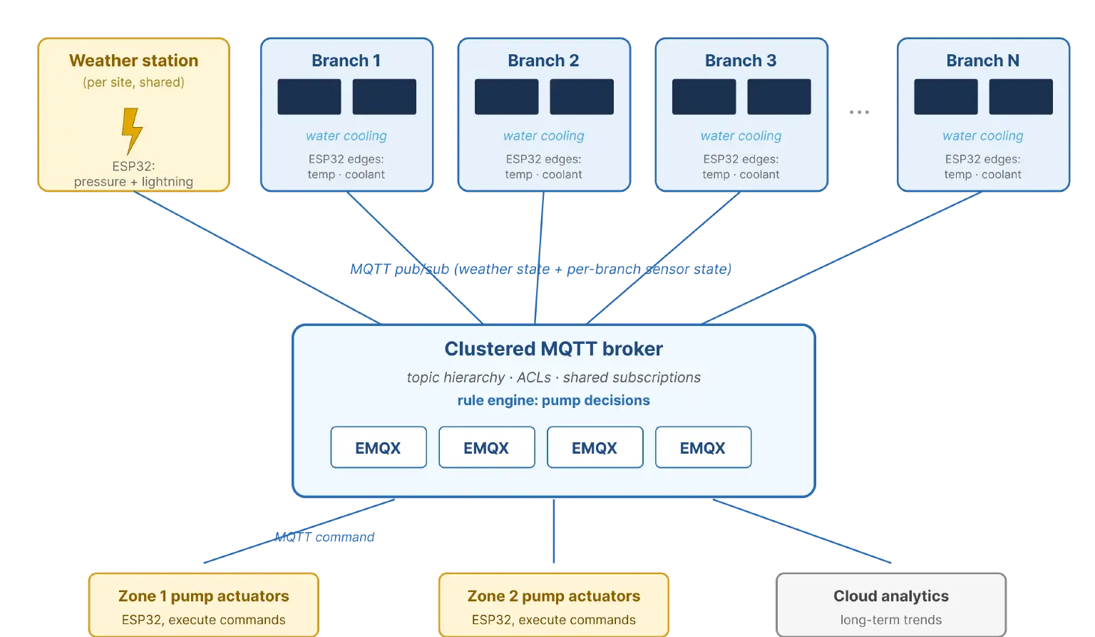
At Production Scale

The paper's four-panel installation fits in a lab. A real deployment spans dozens to hundreds of branches, typically organized into zones with their own fog controllers. The paper's discussion section addresses this directly: "MQTT communication overhead scales approximately linearly with the number of clients and the publish/subscribe model avoids point-to-point connections," and the likely bottleneck sits at the fog layer rather than the broker.

At that scale, the broker runs as a cluster rather than a single process, and the paper's fog-layer decision logic has a natural home inside it. EMQX handles the broker concerns (topic hierarchy, ACLs, shared subscriptions) and evaluates the pump decisions in its rule engine, which collapses the separate fog-layer tier the paper needed in its lab setup.

The Broader Point

A 600 Wp PV branch produced 1.07 units of extra electricity for every unit the cooling system consumed, field-validated across 52 days of real Central European weather. That positive balance came from cooling less often, not harder. Weather-aware suppression of pump activation is what made the cooling worth doing.

In distributed IoT control, what's worth building and what's buildable are the same question. The architecture is not scaffolding for the algorithm. It's part of the algorithm.